
PROCESS INSTRUMENTATION
WHAT IS PROCESS INSTRUMENTATION?
Process instrumentation in the oil and gas industry encompasses the array of sensors, meters, and other measurement and control devices used to monitor, regulate, and manage the operation of processing plants and equipment involved in oil and gas extraction, refining, transportation, and storage.
This technology plays a pivotal role in ensuring operational efficiency, safety, and compliance with environmental and regulatory standards.
Process instruments are designed to measure and control process variables (such as pressure, temperature, flow rate, and level) with high precision and reliability.

Here’s a closer look at its significance:
Key Components of Process Instrumentation
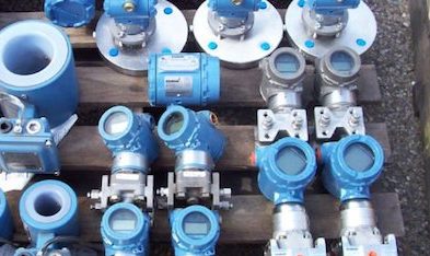
- Sensors and Transmitters: Deployed to measure critical parameters such as pressure, temperature, flow rate, and level within pipes, tanks, and other equipment.
- Control Valves and Actuators: Used to adjust process conditions by controlling the flow of oil, gas, and other substances based on signals received from controllers.
- Controllers: Process controllers interpret data from sensors and transmitters to make decisions and send commands to control devices like valves and actuators.
Functions and Objectives
- Monitoring: Continuous monitoring of process parameters to ensure operations are running within specified limits. This includes tracking the flow of crude oil through pipelines, measuring temperatures in reactors, or monitoring gas pressure in storage facilities.
- Control: Automated or manual adjustment of process variables to maintain optimal operating conditions, improve efficiency, and ensure product quality. For example, adjusting valve positions to regulate the flow rate or pressure.
- Safety: Ensuring the safety of operations by preventing hazardous conditions. Instrumentation detects abnormal conditions like gas leaks, high pressure, or overheating, triggering alarms or automatic shutdowns to mitigate risks.
- Regulatory Compliance: Meeting environmental regulations and standards by monitoring emissions, and effluents, and ensuring the controlled release of substances.
- Data Collection and Analysis: Gathering and analyzing data for operational insights, performance optimization, and predictive maintenance. This helps in identifying trends, improving processes, and reducing downtime.
Importance in the Oil & Gas Industry
In the highly complex and hazardous environment of the oil and gas sector, process instrumentation is vital for:
- Operational Efficiency: Optimizing processes for maximum productivity and minimal waste.
- Quality Assurance: Ensuring the quality of the oil and gas products meets industry standards.
- Environmental Protection: Monitoring and controlling emissions and discharges to minimize environmental impact.
- Economic Performance: Enhancing economic performance by optimizing resource use and reducing operational costs.
Process instrumentation integrates sophisticated technologies, including Internet of Things (IoT) devices and advanced analytics, to create smart, automated systems that enhance decision-making and operational control in the oil and gas industry.
TYPES OF PROCESS INSTRUMENTS
The oil and gas industry relies on a wide array of process instruments to ensure efficient, safe, and compliant operations. These instruments are essential for the monitoring, control, and optimization of various processes involved in the extraction, processing, transportation, and storage of oil and gas. Here are the main types of process instruments used in the industry:
1. Pressure Instruments (Transmitters, Gauges)

2. Temperature Instruments

Temperature Transmitters
Temperature transmitters are devices used in process industries to convert inputs from temperature sensors into standardized output signals that can be easily interpreted by control systems, such as PLCs (Programmable Logic Controllers) or DCS (Distributed Control Systems). These transmitters play a crucial role in temperature monitoring and control, ensuring process stability, efficiency, and safety.
Key Features and Functions:
- Signal Conversion: They convert the low-level signals from temperature sensors (such as thermocouples or RTDs) into higher-level electrical signals (commonly 4-20 mA or 0-10 VDC) that are less susceptible to noise and can be transmitted over long distances.
- Temperature Range and Accuracy: Designed to operate across a wide range of temperatures with high accuracy, making them suitable for various industrial applications.
- Integration and Communication: Many modern temperature transmitters support digital communication protocols (like HART, Foundation Fieldbus, or Profibus), enabling detailed device diagnostics and configuration changes from the control room.
- Environmental Durability: Built to withstand harsh industrial environments, including exposure to high temperatures, pressures, corrosive substances, and vibrations.
Applications:
- Precise monitoring and control of process temperatures in reactors, furnaces, and heat exchangers.
- Safety applications, such as monitoring for overheating conditions in equipment.
Thermocouples
Thermocouples are simple, robust temperature sensors used widely in industrial applications. They consist of two dissimilar metal wires joined at one end (the measuring junction). When the junction experiences a temperature change, a voltage is generated (Seebeck effect) that is proportional to the temperature difference between the measuring junction and the reference junction.
Key Features and Functions:
- Wide Temperature Range: Capable of measuring a broad range of temperatures, from very low to extremely high.
- Fast Response Time: The small mass of the junction allows for rapid response to temperature changes.
- Ruggedness and Simplicity: With no moving parts or need for external power, thermocouples are suited for harsh conditions and are simple to deploy.
- Types and Materials: Various types of thermocouples (Type K, J, T, E, etc.) are available, each made from different materials and optimized for specific temperature ranges and environments.
RTDs (Resistance Temperature Detectors)
RTDs are highly accurate temperature sensors that measure temperature by correlating the resistance of the sensor element with temperature. The sensor element is typically made of platinum (Pt100 or Pt1000), known for its precise and stable resistance-temperature relationship.
Key Features and Functions:
- High Accuracy and Stability: RTDs offer higher accuracy and stability over time compared to thermocouples, making them ideal for applications requiring precise temperature control.
- Linear Response: The resistance of an RTD changes linearly with temperature, simplifying signal processing and calibration.
- Temperature Range: Generally used for measuring temperatures between -200°C and +850°C, covering most industrial applications.
- Sensitivity: RTDs are more sensitive to small temperature changes than thermocouples, providing finer resolution in temperature measurement.
Applications:
- Thermocouples are preferred in high-temperature, rapid-response, or cost-sensitive applications.
- RTDs are chosen for their accuracy and stability in processes requiring precise temperature control, such as in the pharmaceutical and food industries.
Together, temperature transmitters, thermocouples, and RTDs form a comprehensive system for temperature measurement and control, each serving specific needs based on the requirements of accuracy, temperature range, response time, and environmental conditions.
3. Flow Instruments
Flow instruments are crucial components in various industrial processes, designed to measure, monitor, and control the flow rate of liquids, gases, and steam through pipes or other conduits. They ensure optimal operation, safety, and efficiency of systems by providing accurate flow data.

Flow instruments are essential across a wide range of industries, including water and wastewater treatment, oil and gas production, chemical manufacturing, food and beverage processing, and pharmaceuticals. They ensure that fluids are moved, treated, and processed efficiently and safely, meeting both production and regulatory requirements.
The two primary categories of flow instruments are flow meters and flow switches, each serving distinct functions within process control systems:
Flow Meters (e.g., Coriolis, Ultrasonic, Turbine)
Flow meters, also known as flow sensors or flow gauges, are devices that quantify the volume or mass flow rate of a fluid moving through a system. They play a pivotal role in process control by enabling precise measurement of fluid flow, which is critical for various operational needs, including process optimization, quality control, and safety.
Learn more about flowmeters for the oil & gas industry.
Flow Switches
Flow switches are devices designed to trigger an action based on the flow rate of a fluid reaching a specific threshold. Unlike flow meters, which continuously measure the flow rate, flow switches are used for on/off control functions or as safety devices to prevent unwanted conditions such as no flow, low flow, or high flow.
Key Functions of Flow Switches:
- Alarm Activation: Triggering alarms when flow rates fall outside of preset limits.
- Pump Control: Turning pumps on or off based on the detection of flow to prevent dry running or to start backup systems.
- Safety Systems: Activating safety mechanisms in response to flow rate changes, such as shutting down equipment to prevent damage or hazardous conditions.
4. Level Instruments

Level transmitters, gauges, and float switches are essential components in process control, each serving different needs within industrial and utility applications. Transmitters provide continuous and precise electronic monitoring, gauges offer direct visual level indication, and float switches deliver reliable level control. Together, they ensure that level measurement and control tasks are performed efficiently, safely, and in compliance with operational standards.
Let’s delve into the details of this class of process instrumentation:
5. Analytical Instruments

Learn more about devices to monitor the UEL/LEL in the presence of flammable gases.
6. Control Valves
Control valves are special types of valves used to regulate the flow of oil, gas, and other substances based on signals from control systems, adjusting process conditions as needed.
Learn more about control valves for oil & gas processing plants.
7. Safety Instruments
- Gas Detectors: Monitor for hazardous gas leaks, providing early warnings to prevent fires, explosions, and health hazards.
- Emergency Shutdown Systems (ESD): Automatically shut down processes or equipment in response to dangerous conditions, protecting personnel and facilities.
8. Data Acquisition and Signal Conditioning Instruments
- SCADA Systems (Supervisory Control and Data Acquisition): Collect data from various sensors and instruments for monitoring, control, and analysis at a centralized location.
- Signal Converters and Isolators: Ensure that signals from field instruments can be safely and accurately transmitted to control systems.
These instruments form the backbone of the operational technology in the oil and gas industry, enabling companies to achieve their goals of safety, efficiency, and compliance with regulatory standards. Advances in technology, such as wireless communication and IoT devices, are continually enhancing the capabilities and integration of process instrumentation within the industry.
INSTRUMENTS TYPES OF CONTROL SIGNALS: ANALOG, HYBRID, DIGITAL
In the realm of industrial process control and instrumentation, the methods by which instruments communicate and control processes are categorized into three primary types of control signals: analog, digital, and hybrid. Each type of signal offers different characteristics and advantages, making them suitable for various applications depending on the requirements for precision, speed, and complexity of the control system.
The paragraphs below describe the standardized analog pneumatic signals (20 to 100 kPa) and electrical signals (4 to 20 mA), as well as the innovative analog and digital hybrid signals HART (Highway Addressable Remote Transducer) and the state-of-the-art current digital communication protocols commonly called BUS.
ANALOG CONTROL SIGNALS
Analog signals represent data as continuous electrical signals that vary linearly with the physical measurement or control signal. The most common standard for analog signals in process control is the 4-20 mA current loop, where 4 mA represents the lower end of the scale (0% of the measured parameter), and 20 mA represents the upper end (100% of the measured parameter). Voltage signals, such as 0-10V, are also used but are less common due to their susceptibility to noise over long distances.
Advantages:
- Simple and well-understood technology.
- Inherent compatibility with a wide range of equipment.
- Suitable for real-time and continuous control applications.
The traditional most commonly used transmission signal of the type:
- Direct current signals (Table 1): for connection between instruments on long distances (i.e. in the field area)
- Direct voltage signals (Table 2): for connection between instruments on short distances (i.e. in the control room)
| LOWER LIMIT (mA) | UPPER LIMIT (mA) |
| 4 0 | 20 20 |
| (1) Preferential signal | |
Table 1- Standardized signals in direct current (IEC 60381-1)
| LOWER LIMIT (V) | UPPER LIMIT (V) | NOTE |
| 1 – 10 | 5 5 10 + 10 | (1) (1) (1) (2) |
(1) Voltage signals that can be derived directly from normalized current signals (2) Voltage signals that can represent physical quantities of a bipolar nature | ||
Table 2- Standardized signals in direct voltage (IEC 60381-2)
The signal different from 0 (live zero) for the variable at the beginning of the measuring range (true zero), is used for electrical instruments to power the instrument and in general to highlight connection losses (as in the pneumatic instruments).
Moreover, given their characteristics, the current signals are used in the field instrumentation, while the voltage signals are used in the technical and control room instrumentation.
Finally, the current signal concerning the voltage signal has the advantage of not being affected by the length and hence the impedance of the connection line at least up to certain resistance values, as it is illustrated in Figure 1.

Figure 1 – Example of the limit of the operating region for the field instrumentation in terms of its connection resistance Omega to the supply voltage V
Key:
- Vdc = Actual supply voltage in volt
- Vmax= Maximum supply voltage, 30 V in this example
- Vmin= Minimum supply voltage, 10 V in this example
- RL= Max. load resistance in ohm at the actual supply voltage:
- RL <= (Vdc – 10) / 0,02 (in the Example reported in Figure 1)
HYBRID CONTROL SIGNALS
Hybrid signals combine features of both analog and digital signals. A common example of a hybrid signal is the HART protocol (Highway Addressable Remote Transducer), which overlays digital communication on top of a standard 4-20 mA analog signal. This allows for the simultaneous transmission of analog control signals and digital information over the same wiring.
Advantages:
- Compatibility with existing 4-20 mA infrastructure.
- Allows for continuous process control (via the analog signal) and digital communication of additional data.
- Facilitates gradual upgrades from analog to digital systems without a complete overhaul.
More in detail, the HART protocol overlays a digital signal onto the standard analog signal (4-20 mA) by modulating the frequency under the Bell 202 standard. This modulation has an amplitude of +/- 0.5 mA and operates at frequencies detailed in Table 3. Due to the high frequency of the overlaid digital signal, the additional energy introduced is practically negligible, ensuring that this modulation does not interfere with the underlying analog signal.
NOTE: Remember that to operate the HART protocol requires a resistance of 250 ohms in the output circuit!

Table 3 – HART protocol with signals standardized BELL 202
DIGITAL CONTROL SIGNALS
Digital signals represent data in discrete values or binary format (0s and 1s). Digital communication in process control systems is conducted through protocols such as HART (Highway Addressable Remote Transducer), Foundation Fieldbus, Profibus, and Modbus. These protocols allow for two-way communication between devices, enabling not only control but also the transmission of device status, diagnostics, and configuration information.
Advantages:
- Higher accuracy and precision than analog signals.
- Immunity to noise and signal degradation over distance.
- Enhanced capabilities for diagnostics and remote configuration.
The standardization of digital signals was formalized in the late 1990s with the adoption of the International Standard IEC 61158 on Fieldbus Protocol. Despite this, their implementation remains limited, partly because the standard encompasses eight distinct communication protocols. Furthermore, each digital protocol is defined by specific characteristics outlined in Table 4:
- Transmission encoding: Preamble, frame start, transmission of the frame, end of the frame, transmission parity, etc.
- Access to the network: Probabilistic, deterministic, etc.
- Network management: Master-Slave, Producer-Consumer, etc.
| PROTOCOL IEC 61158 | PROTOCOL NAME | NOTE |
| 1 2 3 4 5 6 7 8 | Standard IEC ControlNet Profibus P-Net Fieldbus Foundation SwiftNet WorldFip InterBus | (1) |
| (1) Protocol initially designed as unique standard protocol IEC | ||
Table 4 – Standardized protocols provided for by the International Standard IEC 61158
Finally, Figure 2 shows the geographic path of the measurement signals from the “field” to the “control room” through the “technical room”, where the sorting (also called “marshaling”) takes place and the transformation of the current signal in the voltage signal for the controller (DCS: Distributed Control System) and then through digital signals flow in “control room” for the operator station and video (HMI: Human Machine Interface).

Figure 2 – The typical path of a measurement chain from the field to the control room
POWER SUPPLY FOR PROCESS INSTRUMENTS
- For pneumatic instrumentation: 140 ± 10 kPa (1.4 ± 0.1 bar) for the pneumatic instrumentation (sometimes the normalized pneumatic power supply in English units is still used: 20 psi, corresponding to ≈ 1.4 bar)
- For electrical instrumentation: Continuous voltage: 24 V dc for field instrumentation, Alternating voltage: 220 V ac for control and technical room instrumentation
The connection and transmission signals between the various instruments in the measuring and regulating chains are standardized by the IEC (International Electrotechnical Commission):
- Pneumatic signals (IEC 60382): 20 to 100 kPa (0.2 to 1.0 bar) (sometimes the standardized signal is still in English units: 3 to 15 psi, ≈ 0.21 to 1.03 bar)
- Electrical signals (IEC 60382)
ATTRIBUTES FOR PROCESS INSTRUMENTATION
Understanding the key features of process instrumentation—measurement precision, uncertainty, metrological confirmation, and calibration—is essential for ensuring the optimal performance of such devices operating in industrial processes.
MEASUREMENT PRECISION
Measurement precision of process instruments refers to the consistency and repeatability of the instrument’s measurements under unchanged conditions. It is a measure of how closely repeated measurements of the same quantity agree with each other, rather than the accuracy of the measurements (which refers to how close a measurement is to the true value). In practical terms, precision is about the instrument’s ability to produce the same results again and again over multiple trials without considering whether those results are close to the actual or expected value.
In the context of process instrumentation, high precision is crucial for ensuring stable and reliable process control. For instance, in a chemical manufacturing process, precise temperature control might be necessary to produce a consistent product quality. If a temperature sensor provides precise readings (i.e., consistent with each other) but is not necessarily accurate (i.e., close to the actual temperature), the process can still be controlled effectively as long as the deviation from the true value is known and consistent.
However, it’s important to note that while precision is essential for the reliability and consistency of process operations, it is equally important to calibrate instruments regularly to ensure their measurements are both precise and accurate. Precision alone does not guarantee that an instrument accurately reflects the true value of the measured variable, but it is a critical component of overall measurement quality in industrial processes.
The concept of measurement precision is defined in various ways by different entities involved in the specification of process instruments:
- according to ISO-IMV (International Metrology Vocabulary): “…closeness of agreement between indications or measured quantity values obtained by replicate measurements on the same or similar objects under specified conditions”;
- according to IEC-IEV (International Electrotechnical Vocabulary): “..quality which characterizes the ability of a measuring instrument to provide an indicated value close to a true value of the measurand” (Note: call in this case, however, not Precision but Accuracy);
- or we could deduce the following practical definition from the previous ones:“…by testing a measuring instrument under conditions and with specified procedures, the maximum positive and negative deviations from a specified characteristic curve (usually a straight line)”.
Therefore, the concept of linearity is also inherent in the measurement precision term (which is currently very limited in the digital instrumentation), while the concept of hysteresis is not included (although this is considered, as it is included within the maximum positive and negative deviations found).
Furthermore, the concept of repeatability of the measurement is not included (which is instead considered in the case of verification of precision over several measuring cycles.
Therefore, in the practical verification of the precision of the measuring instruments with a single up and down measurement cycle (generally conducted for instruments with hysteresis, such as pressure gauges, pressure transducers, load cells, etc.) a calibration curve is obtained of the type found in Figure 1, where we can deduce the concept of tested accuracy (accuracy measured) that must be included within the so-called nominal accuracy (accuracy rated) or the limits within which the imprecision of an instrument is guaranteed by its specification.
The metrological confirmation is the verification that the measuring instrument keeps the accuracy and uncertainty characteristics required by the measurement process over time.
Sometimes this concept of imprecision for some common types of instruments (such as gauges, resistance thermometers, thermocouples, etc.) is also called precision or accuracy class, which according to the International Reference Vocabularies ISO-IMV and IEC-IEV: “class of measuring instruments or measuring systems that meet stated metrological requirements that are intended to keep measurement errors or instrumental measurement uncertainties within specified limits under specified operating conditions” (ie, the accuracy measured must be less than accuracy rated: See also Figure 1).

Figure 1 – Exemplification of measurement accuracy concepts
MEASUREMENT UNCERTAINTY
The measurement uncertainty of the measuring instrument is a new concept that takes into account during the calibration not only the errors or deviations found but also its resolution of indication as well as the uncertainty of the measurement standard used in the calibration itself.
The concept of measurement uncertainty is defined in various ways by different entities involved in the specification of process instruments:
- according to ISO-IMV (Internat. Metrology Vocabulary): “non-negative parameter characterizing the dispersion of the quantity values being attributed to a measurand, based on the information used”;
- according to ISO-GUM (Guide to Uncertainty of the Measurement): “result of the estimation that determines the amplitude of the field within which the true value of a measurand must lie, generally with a given probability, that is, with a determined level of confidence”.
From the above definitions, we can deduce two fundamental concepts of measurement uncertainty:
- Uncertainty is the result of an estimate, which is evaluated according to the following two types:
- Category A: when the evaluation is done by statistical methods, that is through a series of repeated observations, or measurements.
- Category B: when the evaluation is done using methods other than statistical, that is, data that can be found in manuals, catalogs, specifications, etc.
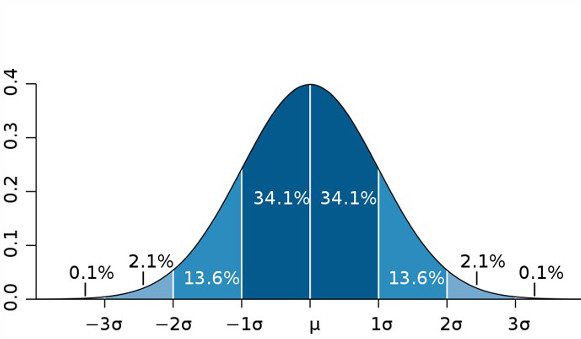
2. The uncertainty of the estimate must be given with a certain probability, which is normally provided in the three following expressions (see also Table 1):
- Standard uncertainty (u): at the probability or confidence level of 68% (exactly 68.27%).
- Combined uncertainty (uc): the standard uncertainty of measurement when the result of the estimate is obtained using the values of different quantities and corresponds to the summing in quadrature of the standard uncertainties of the various quantities relating to the measurement process.
- Expanded uncertainty (U): uncertainty at the 95% probability or confidence level (exactly 95.45%), or 2 standard deviations, assuming a normal or Gaussian probability distribution.
Table 1- Main terms & definitions related to measurement uncertainty according to ISO-GUM
Standard uncertainty u(x) (a)
The uncertainty of the result of measurement expressed as a standard deviation u(x) º s(x)
Type A evaluation (of uncertainty)
Method of evaluation of uncertainty by the statistical analysis of a series of observations
Type B evaluation (of uncertainty)
Method of evaluation of uncertainty by means other than the statistical analysis of a series of observations
Combined standard uncertainty uc(x)
The standard uncertainty of the result of measurement when that result is obtained from the values of several other quantities, equal to the positive square root of a sum of terms, the terms being the variances or covariances of these other quantities weighted according to how the measurement result varies with changes in these quantities
Coverage factor k
The numerical factor is used as a multiplier of the combined standard uncertainty to obtain an expanded uncertainty (normally is 2 for probability @ 95% and 3 for probability @ 99%)
Expanded uncertainty U(y) = k . uc(y) (b)
Quantity defining an interval about the result of a measurement that may be expected to encompass a large fraction of the distribution of values that could reasonably be attributed to the measurand (normally obtained by the combined standard uncertainty multiplied by a coverage factor k = 2, namely with the coverage probability of 95%)
(a) The standard uncertainty u (y), ie the mean square deviation s (x), if not detected experimentally by a normal or Gaussian distribution, can be calculated using the following relationships:
u(x) = a/Ö3, for rectangular distributions, with an amplitude of variation ± a, eg Indication errors
u(x) = a/Ö6, for triangular distributions, with an amplitude of variation ± a, eg Interpolation errors
(b) The expanded measurement uncertainty U (y) unless otherwise specified, is to be understood as provided or calculated from the uncertainty composed with a coverage factor 2, ie with a 95% probability level.
METROLOGICAL CONFIRMATION
Metrological confirmation for process instrumentation is the process of ensuring that measuring instruments are suitable for their intended purposes and meet all the specified requirements. This involves a series of activities, including calibration, verification, and validation, to confirm that the instruments perform accurately and reliably within the context of their operational environment and applications. The goal of metrological confirmation is to provide confidence in the measurements obtained from these instruments, which are critical for process control, quality assurance, and compliance with regulatory standards.
The metrological confirmation is the routine verification and control operation that confirms that the measuring instrument (or equipment) maintains the accuracy and uncertainty characteristics required for the measurement process over time.
By metrological confirmation, we mean according to ISO 10012 (Measurement Management System): a “set of interrelated or interacting elements necessary to achieve metrological confirmation and continual control of measurement processes”, and generally includes:
- instrument calibration and verification;
- any necessary adjustment and the consequent new calibration;
- the comparison with the metrological requirements for the intended use of the equipment;
- the labeling of successful positive metrological confirmation.
The metrological confirmation must be guaranteed through a measurement management system which essentially involves the phases of Table 1.
| NORMAL PHASES | PHASES IN CASE OF ADJUSTMENT | PHASES IN CASE OF IMPOSSIBLE ADJUSTMENT |
| 0. Equipment scheduling | ||
| 1. Identification need for calibration | ||
| 2. Equipment calibration | ||
| 3. Drafting of calibration document | ||
| 4. Calibration identification | ||
| 5. There are metrological requirements? | ||
| 6. Compliance with metrological req. | 6a. Adjustment or repair | 6b. Adjustment Impossible |
| 7. Drafting document confirms | 7a. Review intervals confirm | 7b. Negative verification |
| 8. Confirmation status identification | 8a. Recalibration phase (2 to 8) | 8b. State of identification |
| 9. Satisfied need | 9a. Satisfied need | 9b. Need not satisfied |
Table 1 – Main phases of the metrological confirmation (ISO 10012)
Table 1 highlights three possible paths of metrological confirmation:
- the left path that normally achieves the satisfaction of the positive outcome of the metrological confirmation without any adjustment of the instrument in confirmation to phase 6;
- the first left path and then the middle one from phase 6a to 9a, in case of positive adjustment or repair of the instrument in confirmation and whose recalibration satisfies the confirmation: therefore, in this case, it will be necessary to reduce only the confirmation interval;
- the first path on the left and then the right from phase 6b to 9b, in case of negative adjustment or repair of the instrument in confirmation, which does not satisfy the result of the confirmation: therefore the instrument must be downgraded or alienated.
Metrological confirmation can usually be accomplished and fulfilled in two ways:
- Comparing the Maximum Relieved Error (MRE) with the Maximum Tolerated Error (MTE), ie: MRE <= MTE
- Comparing the Max. Relieved Uncertainty (MRU) with Tolerated Uncertainty (MTU, ie: MRU <= MTU
Concerning the previous articles, and taking into consideration the one on the Calibration, related to the evaluation of the calibration results in terms of Error and Uncertainty of a manometer, respectively equal to:
- MRE: ±05 bar
- MRU: 066 bar
if the maximum error and tolerated uncertainty were both 0.05 bar, then the manometer if evaluated in terms of MRE is compliant, while if evaluated in terms of MRU it is not compliant, and therefore it should follow path 2 of Table 1, or path 3; if it does not fall into it is then downgraded.
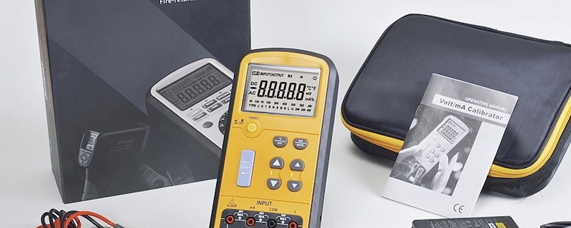
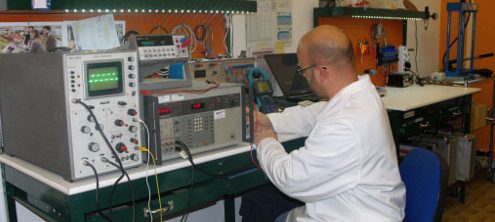
INSTRUMENTS CALIBRATION
Instrumentation calibration is the operation to obtain under specified conditions, the relationship between the values of a measurand and the corresponding output indications of the instrument in calibration.
By calibration, we mean:
- according to ISO-IMV (International Metrology Vocabulary): “operation that, under specified conditions, in a first step, establishes a relation between the quantity values with measurement uncertainties provided by measurement standards and corresponding indications with associated measurement uncertainties and, in a second step, uses this information to establish a relation for obtaining a measurement result from an indication”;
- or we could deduce the following practical example from the previous one: “operation performed to establish a relationship between the measured quantity and the corresponding output values of an instrument under specified conditions”.
Calibration should not be confused with adjustment, which means: “set of operations carried out on a measuring system so that it provides prescribed indications corresponding to given values of a quantity to be measured (ISO-IMV).
Hence, the adjustment is typically the preliminary operation before the calibration, or the next operation when a de-calibration of the measuring instrument is found.
Calibration should be performed on 3 or 5 equidistant measuring points for increasing (and decreasing) values in the case of instruments with hysteresis phenomena: eg manometers):
Figure 1 presents the calibration setup, while Table 1 presents the calibration results.

Figure 1 – Calibration setup of a manometer
| |||||||||||||||||||||||||||||||||||||||||
| Table 1 – Calibration Results | |||||||||||||||||||||||||||||||||||||||||
From the calibration results shown in Table 1, the metrological characteristics of the manometer (or pressure gauge) can be obtained in terms of:
- Measurement Accuracy: that is, maximum positive and negative error: ± 0.05 bar
- Measurement Uncertainty: or instrumental uncertainty that takes into account the various factors related to the calibration, namely:
Iref Uncertainty of the reference standard 0.01 bar (supposed)
Emax Max error of measurement relieved 0.05 bar
Eres Error of resolution of the manometer 0.05 bar
from which the composed uncertainty uc can be derived from the following relation:
and then the extended uncertainty (U), at a 95% confidence level (ie at 2 standard deviations):
![]()
NOTE:
Obviously, the measurement uncertainty of the manometer (usually called instrumental uncertainty) is always higher than the measurement accuracy (because it also takes into account the error of resolution of the instrument in calibration and the uncertainty of the reference standard used in the calibration process).
PDF – Traceability & Calibration Handbook (Prof. Brunelli)
![]() Traceability&Calibration Handbook (Process Instrumentation)
Traceability&Calibration Handbook (Process Instrumentation)
Book – Instrumentation Manual (Prof. Brunelli)
Buy the “Instrumentation Manual” on Amazon.
The book illustrates:
- Part 1: illustrates the general concepts of industrial instrumentation, the symbology, the terminology and calibration of the measurement instrumentation, the functional and applicative conditions of the instrumentation in normal applications and with the danger of explosion, as well as the main directives (ATEX, EMC, LVD, MID, and PED);
- Part 2: this part of the book deals with the instrumentation for measuring physical quantities: pressure, level, flow rate, temperature, humidity, viscosity, mass density, force and vibration, and chemical quantities: pH, redox, conductivity, turbidity, explosiveness, gas chromatography, and spectrography, treating the measurement principles, the reference standard, the practical executions, and the application advantages and disadvantages for each size;
- Part 3: illustrates the control, regulation, and safety valves and then simple regulation techniques in feedback and coordinates in feedforward, ratio, cascade, override, split range, gap control, variable decoupling, and then the Systems of Distributed Control (DCS) for continuous processes, Programmable Logic Controllers (PLC) for discontinuous processes and Communication Protocols (BUS), and finally the aspects relating to System Safety Systems, from Operational Alarms to Fire & Gas Systems, to systems of ESD stop and finally to the Instrumented Safety Systems (SIS) with graphic and analytical determinations of the Safety Integrity Levels (SIL) with some practical examples.


One Response
The Calibration Process for the Ultrasonic Flaw Detector Thickness measurement is not the sole consideration.
The Calibration Process for the Ultrasonic Flaw Detector Thickness measurement is not the sole consideration.
https://www.eurocaltech.com/service-details.php?recId=25
Calibration is a crucial process for non-destructive testing professionals to ensure the accuracy and precision of their ultrasonic flaw detector. It involves setting the measuring instrument with a standard unchanging reference material that meets certain specifications. This process often occurs in two stages: manufacturer calibration, where the flaw detector meets the standard manufacturing specification outlined in the relevant code, and user calibration, which ensures the detector meets the specification for the anticipated flaw to be detected.
The most important reason for calibrating ultrasonic flaw detectors is to ensure that it is accurate and void of errors. Over time, the cumulative margin of error increases, and the inaccuracy becomes big and beyond acceptable tolerance levels. Periodically calibrating your ultrasonic flaw detector reduces this margin of error to the barest minimum without overtly affecting the result.
There are three ways to set up for an ultrasonic flaw detector calibration: zero offset calibration, material velocity calibration, and auto calibration. Zero offset calibration considers the time elapsed during wave travel before entering the test sample and equates it to the time elapsed as it travels through a layer of the test sample. Material velocity calibration depends on the material to be inspected and the ambient temperature obtainable during the setup. Auto calibration requires specific settings to be in place before calibration, including using the ultrasonic velocity tables to adjust material velocity values closer to real values, setting delay and zero offset values to zero, and adjusting the speed of two similar signal reflectors sending two separate signals from different distances.
Ultrasonic flaw detectors typically require three calibration processes: velocity/zero calibration, reference calibration, and calibration certification. Velocity/zero calibration converts time to distance measurements using the speed of sound in test materials to program the flaw detector. It considers the dimensions measured by the flaw detector, including the distance and thickness of the material, using precisely timed echoes. The accuracy of this calibration depends on the careful measures taken during the calibration exercise, and errors might occur in the readings if the calibration is not carefully and correctly done.
Reference calibration uses similar materials or test blocks as reference standards to set up a testing operation. For ultrasonic flaw detectors, the signal’s amplitude received from standard references is usually used for this type of calibration. User-defined procedures often provide the details required for reference calibration used for specific tests.
Calibration certification involves documenting an ultrasonic flaw detector’s linearity and measurement accuracy given specific test conditions. This measurement accuracy is often juxtaposed with the manufacturer’s given tolerances. Distance and amplitude certifications are given for ultrasonic flaw detectors, but the certification must still follow relevant codes and standards such as EN 12668 or E-317.
To calibrate an ultrasonic flaw detector, three steps are used: setting the probe in position A with the right coupling, adjusting the range and sound velocity, and setting the angle probe for angle. The speed/delay is instantly set and calibrated with the actual velocity also computed. The angle probe for angle is set in position C with the right coupling, and the aperture, depth of hole, and calibration type are entered. The gain is set to the correct value, and the probe should be adjusted to the highest echo conforming to a 50mm hole.